Microsoft Excel provides various number formatting options which allows you to easily format numbers as currency, dates, percentages, time and even fractions. Occasionally you may run into a situation where the predefined number formats do not suit your needs for a range of data. This is where custom number formats can help you to create your own formats.
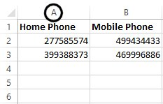
A perfect example of this is when entering phone numbers with an area code, or when entering mobile (cell) phone numbers. In Australia, our mobile or cell phone numbers begin with a zero (0) as do our home or business phone numbers. When you enter a number into any cell, beginning with a zero (0), Excel will drop the zero at the beginning but leave the remaining digits behind. This is very frustrating for many users and so there is a way we can fix this using custom number formats. We can essentially force Excel to add in the extra digit that it keeps discarding and create our own unique way to format various types of numbers including currency and dates.
Create a custom number format
There are two types of format code characters we are going to use in this exercise: the hash symbol (#) and the zero (0).
The hash symbol will allow you to specify the placement of any significant digits within your values e.g. each digit displayed in our phone numbers is considered significant therefore the hash symbol will let us show Excel where we want those digits placed in the formatting.
The zero (0) placeholder, however, displays insignificant zeros where a number does not have enough digits to fill in the format.
To create a custom number format, follow these steps:
- Highlight the entire column you wish to format with a custom number format by clicking on the column heading

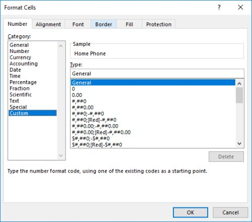
- Right mouse click on the column and choose Format Cells or press Ctrl + 1 on the keyboard
- From the Number tab select Custom

- Excel will display a list of available custom formats, you can use these as a guide for creating other custom formats however for this exercise we will create our own format
- You will see a lot of the custom formats have combinations of zero (0) and the hash symbol (#)
- Place your cursor in the Type field and enter 0# #### #### to represent a phone number with a 2-digit area code and 2 groups of 4 digits, don’t forget the spaces
- Click OK
- The phone numbers will now be reformatted to the new custom format

- Test out the custom number by entering a new number into the next blank cell (A4), don’t type any spaces and you can even leave out the first zero from the area code and Excel will adjust the format for you
TIP: If the new entry does not format as expected you may have only selected the individual cells which contained the phone numbers instead of selecting the entire column.
- Repeat the process for any remaining columns. The custom format for a mobile number would be 0### ### ###.

I hope this gives you a great introduction to creating custom number formats in Excel.
Reference: https://www.thetraininglady.com/custom-number-formats/
