
Conditional formatting is one of my favourite parts of Excel. I am a very visual person and would much rather look at colour charts or visual representations of data to give me a sense of what I’m looking at. Conditional formatting is the easiest way to achieve this result.
I am always surprised how often participants in training are manually formatting specific cells with different colours to highlight their values, rather than letting Excel do the work for them.
Conditional formatting will allow you to apply “rules” or “conditions” to a range of cells and based on the rules you can then format the content. There are many pre-defined rules available but you can also define your own custom rules to suit your individual needs.
Apply conditional formatting
To apply conditional formatting, follow these steps:
- Highlight the entire column(s) or row(s) you want the rule to apply to, you can also use the keyboard shortcut of Ctrl + Spacebar.
- To select multiple adjacent columns simply click and drag the mouse to the left or right to highlight the additional columns

- From the Home tab on the Ribbon select the Conditional Formatting button within the Styles group

- Now to choose the type of conditional formatting you wish to use. If you wish to highlight cells based on a value, such as highlighting cells with a value greater than 10, then you can use the pre-defined options available in the Highlight Cell Rules. The Top/Bottom Rules option also has predefined options.
- For this example, I’m going to select Highlight Cell Rules > Greater Than
- The Greater Than dialog box will appear:
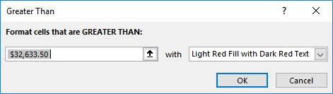
- Excel will automatically put a value in the value field, to change this simply type straight over the top or you can use cell references here to reference a cell in your worksheet which contains the value you want to use.
- Enter the value you’d like to highlight for this column. For this, I want to highlight any values which are greater than 38200 so I enter the value into the field.
- Using the drop-down menu select the type of formatting you want to use, Excel provides some predefined options so you can use one of those or choose Custom Format if you wish to format cells using your own formatting choices.
- You will see that Excel is showing you a live preview of the result in the data on your worksheet.
- Once you are happy click OK. Remember you can always go back and change these settings later.
- Any data which meets the criteria you have set in the conditional formatting rule will now be highlighted:

Edit a conditional formatting rule
If you need to edit an existing rule, follow these steps:
- Highlight the column or range of data you need to change and click the Conditional Formatting button again from the Home tab, then choose Manage Rules.
- The Conditional Formatting Rules Manager will appear:

- If you want to view all conditional formatting rules set up in your entire worksheet, click on the Show formatting rules for drop-down menu at the top of the dialog and choose This worksheet.
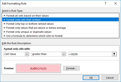
- Select the rule you wish to edit from the list and click Edit Rule.
- You will now see the specifics of the rule you have created, including the type of formatting which will be applied, you can edit any aspect of these settings.
- Once complete click OK to close the dialog box.
- Now click OK on the Conditional Formatting Rules Manager window to return to your worksheet.
- You will now see the changes applied to your rule.
There are some amazing options in conditional formatting so it’s worth taking the time to experiment with the other options. I personally find the Top/Bottom rules are very useful as are the Data Bars and Icon Sets.
Reference: https://www.thetraininglady.com/conditional-formatting-excel/